Quantification of the multifaceted impacts of atmospheric environmental variations on public health, solar energy, and wind energy.
1. Public health
To quantify the impacts of fine particulate matter (PM2.5) on public health, only PM2.5 concentrations ($\mu$g m$^{-3}$) are needed, as part of a collaboration with BNU and XMU. Link
2. Solar energy
As defined and used in most (though not all) studies, capacity factor (CF, unitless) is a dimensionless magnitude accounting for the performance of the PV cells with respect to their nominal power capacity according to the actual ambient conditions. Therefore, CF multiplied by the nominal installed watts of PV power capacity gives instantaneous PV power production.
2.1. My gc-pvlib-Li.py that can consider both PM dimming and soiling:
Refs: Bergin et al., ES&TL, 2017, Li et al., NS, 2020, Yao and Palmer, ES&T, 2022, Yao et al., ES&T, 2025, Yin et al., CEE, 2026, etc.
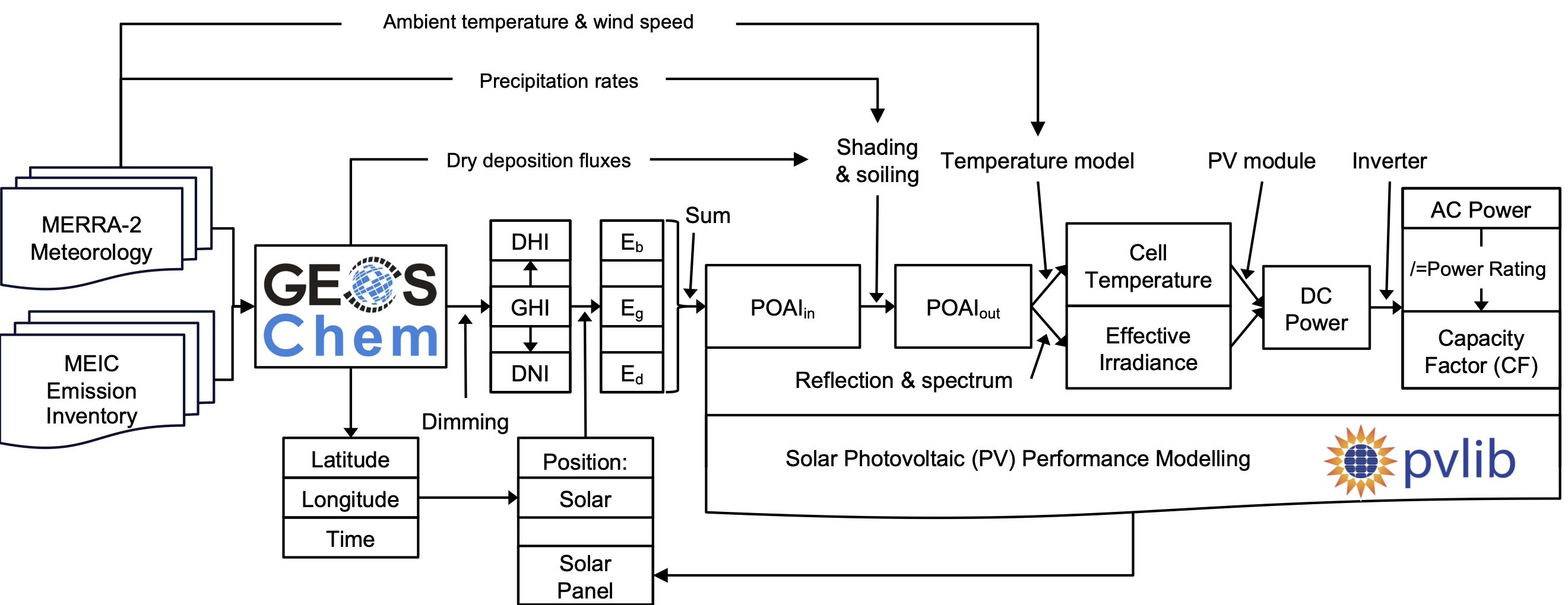
Each data record must contain coordinates for latitude, longitude, and UTC time (must be every three hours or more frequently to facilitate the calculation of solar position for tracking and DNI/DHI $\leftarrow$ GHI), as well as the following variables:
$GHI$: Global Horizontal Irradiance (W m$^{-2}$)
$DNI$: Direct Normal Irridance (W m$^{-2}$)
$DHI$: Diffuse Horizontal Irradiance (W m$^{-2}$)
Note that models like GEOS-Chem may provide only $GHI$; in such cases, we use the Erbs model (or similar methods) to estimate $DNI$ and $DHI$ from $GHI$.
$pressure$: Air pressure (Pa) to help determine altitude from sea level (m) and to adjust solar position and air mass estimates.
$albedo$: reflectivity of the ground surface (unitless)
$GraDepFlux\_spe$: gravitational deposition flux of a specific aerosol species (kg m$^{-2}$ s$^{-1}$ integrated over time $\rightarrow$ g m$^{-2}$)
$TurDepFlux\_spe$: turbulent deposition flux of a specific aerosol species (kg m$^{-2}$ s$^{-1}$ integrated over time $\rightarrow$ g m$^{-2}$)
We distinguish between gravitational and turbulent deposition fluxes, as gravitational deposition is reduced on tilted panels whereas turbulent deposition is not. These fluxes may also be derived from the product of deposition velocities ($GraDepVel\_spe$ and $TurDepVel\_spe$) and near-surface aerosol concentrations ($AerMass$). For aerosol species, we require at least a separation between secondary inorganic aerosols (sulfate + nitrate + ammonia), black carbon, organic carbon, and dust because of their different optical effects on solar panels. More detailed speciation is acceptable, as it can be aggregated within the coupling code. If gravitational and turbulent deposition fluxes/velocities cannot be readily distinguished, we consider separate them using aerosol composition. For instance, coarse dust particles are predominantly associated with gravitational settling, whereas other species are mainly governed by turbulent deposition. Relevant supporting literature will be required, though.
$precipitation\_rates$: precipitation rates at the ground (mm h$^{-1}$)
$temp\_air$: Air temperature (also known as dry-bulb temperature) ($^{\circ}$C)
$wind\_speed$: Wind speed at a height of 10 meters (m s$^{-1}$)
Among the five meteorological variables listed above, $temp\_air$ and $pressure$ are primarily used to adjust solar position and air mass estimates, which may influence irradiance (for example, the perez sky diffuse model requires air mass as an input), but should only to a limited extent. $albedo$ changes very slowly; however, because it directly converts $GHI$ to $E_b$, it has a strong impact on irradiance. $precipitation\_rates$ affects soiling and therefore irradiance. $temp\_air$ and $wind\_speed$ mainly affect cell temperature rather than irradiance.
To isolate the effects of changing meteorological conditions on irradiance alone, we can keep $temp\_air$ and $wind\_speed$ the same as in the CTRL case while varying the other variables as needed. The only drawback of this approach is that $temp\_air$ may slightly affect the solar position, and therefore irradiance, calculations. However, this impact should be minimal (see discussion here). Hence, we may not supply an alternative $temp\_air$ source specifically for solar position calculations in both gc-pvlib-Li.py and modelchain.py, as outlined below:
solar_position = location.get_solarposition(index,
                                            pressure=pressure,
                                            temperature=temp_air)

---

# build kwargs for solar position calculation
try:
    press_temp = _build_kwargs(['pressure', 'temp_air'], weather)
    press_temp['temperature'] = press_temp.pop('temp_air')
except KeyError:
    pass
self._prep_inputs_solar_pos(kwargs=press_temp) # press_temp => kwargs=press_temp for readability.
$grid\_indices$: indices of the grid cells included in the parallel calculations. This is optional but can improve performance by restricting computations to selected areas (e.g., land grids only).
| Variable | Description | Units |
|---|---|---|
| $GHI$ | Global Horizontal Irradiance | W m$^{-2}$ |
| $DNI$ | Direct Normal Irridance | W m$^{-2}$ |
| $DHI$ | Diffuse Horizontal Irradiance | W m$^{-2}$ |
| $pressure$ | Air pressure | Pa |
| $albedo$ | Reflectivity of the ground surface | 1 |
| $GraDepFlux\_spe$ | Gravitational deposition flux of a specific aerosol species | kg m$^{-2}$ s$^{-1}$ integrated over time $\rightarrow$ g m$^{-2}$ |
| $TurDepFlux\_spe$ | Turbulent deposition flux of a specific aerosol species | kg m$^{-2}$ s$^{-1}$ integrated over time $\rightarrow$ g m$^{-2}$ |
| $precipitation\_rates$ | Precipitation rates at the ground | mm h$^{-1}$ |
| $temp\_air$ | Air temperature (also known as dry-bulb temperature) | $^{\circ}$C |
| $wind\_speed$ | Wind speed at a height of 10 meters | m s$^{-1}$ |
| $grid\_indices$ | Indices of the grid cells included in the parallel calculations | N/A |
2.2. Alternative empirical methods that can only consider PM dimming:
On the other hand, most studies (e.g. Jerez et al., NC, 2015, Feron et al., NS, 2020, Lei et al., NCC, 2023, Qin et al., NG, 2024) examing the impacts of climate change and/or carbon neutrality on solar PV efficiency or capacity factor ($CF$, unitless) have primarily focused on the effects of PM dimming, while neglecting soiling. In such cases, only downward shortwave radiation ($I$, W m$^{-2}$), ambient temperature at 2 m ($T_{2m}$, $^{\circ}$C), and wind speed at 10 m ($u_{10m}$, m s$^{-1}$) are required:
\[CF = P_R \frac{I}{I_{STC}},\]where STC refers to the standard test conditions ($I_{STC}=1000$ W m$^{-2}$), those for which the nominal capacity of a PV devive is determined as its measured power output, and $P_R$ is the so-called performance ratio, formulated to account for changes of the PV cells efficiency due to changes in their temperature as:
\[P_R = 1 - \gamma (T_{cell} - T_{STC}),\]where $T_{cell}$ in the PV cell temperature, $T_{STC}$=25 $^{\circ}$C and $\gamma$ is taken here as 0.005 $^{\circ}$C$^{-1}$, considering the typical response of monocrystalline silicon solar panels. Finally, $T_{cell}$ is modelled considering the effects of $T_{2m}$, $I$, and $u_{10m}$ on it as:
\[T_{cell} = c_1 + c_2 T_{2m} + c_3 I - c_4 u_{10m},\]with $c_1 = 4.3^{\circ}C$, $c_2=0.943$, $c_3=0.028^{\circ}$C (W m$^{-2}$)$^{-1}$, $c_4=1.528^{\circ}$C (m s$^{-1}$)$^{-1}$.
Hence, if ambient conditions ($I$, $T_{2m}$ and $u_{10m}$) correspond to the STCs, $CF$ equals 1 and PV power production reaches the rated value. If they are so that $T_{cell}$ is higher (lower) than 25 $^{\circ}$C and/or $I$ lower (higher) than 1,000 W m$^{−2}$, $CF$ will be lower (higher) than the unit and the PV power output will be lower (higher) than the nominal power of the module.
| Variable | Description | Units |
|---|---|---|
| $I$ | Downward shortwave radiation | W m$^{-2}$ |
| $T_{2m}$ | Ambient temperature at 2 m | $^{\circ}$C |
| $u_{10m}$ | Wind speed at 10 m | m s$^{-1}$ |
| $I_{STC}$ | Shortwave radiation on PV panels under standard test conditions (1000 W m$^{-2}$) | W m$^{-2}$ |
| $P_R$ | Performance ratio | 1 |
| $T_{cell}$ | Cell temmperature | $^{\circ}$C |
| $T_{STC}$ | Cell temmperature under standard test conditions (25 $^{\circ}$C) | $^{\circ}$C |
| $\gamma$ | 0.005 | $^{\circ}$C$^{-1}$ |
| $c_1$ | 4.3 | $^{\circ}$C |
| $c_2$ | 0.943 | 1 |
| $c_3$ | 0.028 | $^{\circ}$C (W m$^{-2}$)$^{-1}$ |
| $c_4$ | 1.528 | $^{\circ}$C (m s$^{-1}$)$^{-1}$ |
3. Wind energy
In Qin et al., NG, 2024, the wind capacity factor is simply derived from a piecewise function of the wind speed at 100 m ($u_{100m}$, m s$^{-1}$):
\[CF = \begin{cases} 0, & u_{100m} < u_{cut-in}~\text{or}~u_{100m} > u_{cut-out} \\ \frac{u_{100m}^3 - u_{cut-in}^3}{u_{rated}^3 - u_{cut-in}^3}, & u_{cut-in} \leq u_{100m} \leq u_{rated} \\ 1, & u_{rated} < u_{100m} \leq u_{cut-out} \end{cases}\]where $u_{cut-in}$ is the cut-in wind speed (3 m s$^{-1}$), below which the wind power turbine will not rotate; $u_{cut-out}$ is the cut-out wind speed (25 m s$^{-1}$), above which the wind power turbine will shut down for safety reasons; and $u_{rated}$ is the rated wind speed (12 m s$^{-1}$), at which the turbine reaches its nominal power output. To derive $u_{100m}$ from the wind speed at 10 m ($u_{10m}$, m s$^{-1}$), the authors use the wind profile formula:
\[u_{100m} = u_{10m} \left( \frac{100}{10} \right)^{\alpha},\]where the scaling factor $\alpha$ represents how quickly the wind decays towards the ground, and is offten approximated as a constant of 0.143 over land surfaces.
| Variable | Description | Units |
|---|---|---|
| $u_{10m}$ | Wind speed at 10 m | m s$^{-1}$ |
| $u_{100m}$ | Wind speed at 100 m | m s$^{-1}$ |
| $\alpha$ | 0.143 | 1 |
| $u_{cut-in}$ | Cut-in wind speed (3 m s$^{-1}$), below which the wind power turbine will not rotate | m s$^{-1}$ |
| $u_{cut-out}$ | Cut-out wind speed (25 m s$^{-1}$), above which the wind power turbine will shut down for safety reasons | m s$^{-1}$ |
| $u_{rated}$ | Rated wind speed (12 m s$^{-1}$) | m s$^{-1}$ |